Spike width versus cortical depth in the mouse isocortex
An exploratory–confirmatory analysis of the IBL Brain Wide Map
1 Original question
Is there a relationship between the spike width and the cortical depth (as a percentage of the cortical layers) in the IBL dataset? The spike width is the peak-to-trough duration from the waveform features.
2 Introduction
The extracellular spike waveform is the main handle on cell type in large-scale extracellular recordings. Narrow spikes (peak-to-trough ≲ 0.4 ms) are mostly fast-spiking, parvalbumin-expressing interneurons, while broad spikes are mostly pyramidal cells (Barthó et al. 2004). The mapping is imperfect: some large pyramidal cells have thin spikes (Vigneswaran et al. 2011), and axonal and dendritic signals have distinct waveform shapes (Jia et al. 2019).
Cell types are not distributed uniformly across cortical layers. Interneuron classes have characteristic laminar distributions (Tremblay et al. 2016; Kim et al. 2017), and spike-waveform and firing properties differ between layers of the mouse cortex (Senzai et al. 2019). If spike width tracks cell type, its distribution should change with depth.
The IBL Brain Wide Map (International Brain Laboratory 2025) gives Neuropixels recordings from many cortical areas and mice. These recordings are localized in the Allen Common Coordinate Framework (Wang et al. 2020), which makes a laminar survey of spike width across the isocortex possible.
3 Refinement of the question
3.1 Data
Data come from the bwm_ephys v1.2.1 derived dataset (full cluster table and peak-channel mean waveforms). Units are good units (IBL QC label = 1) whose Allen region is a descendant of Isocortex: 12,982 units, 351 insertions, 118 mice.
Mice are the independent statistical unit. A seeded random 20 % of mice formed the exploration set (24 mice, 68 insertions, 1,892 units). The remaining 94 mice formed the confirmation set (283 insertions, 11,090 units), which was not examined until the test plan was locked.
3.2 Spike width
Spike width is the stored peak_to_trough_duration: the time from the main (negative) peak of the peak-channel mean waveform to the following positive trough, sampled at 30 kHz (33 µs resolution).
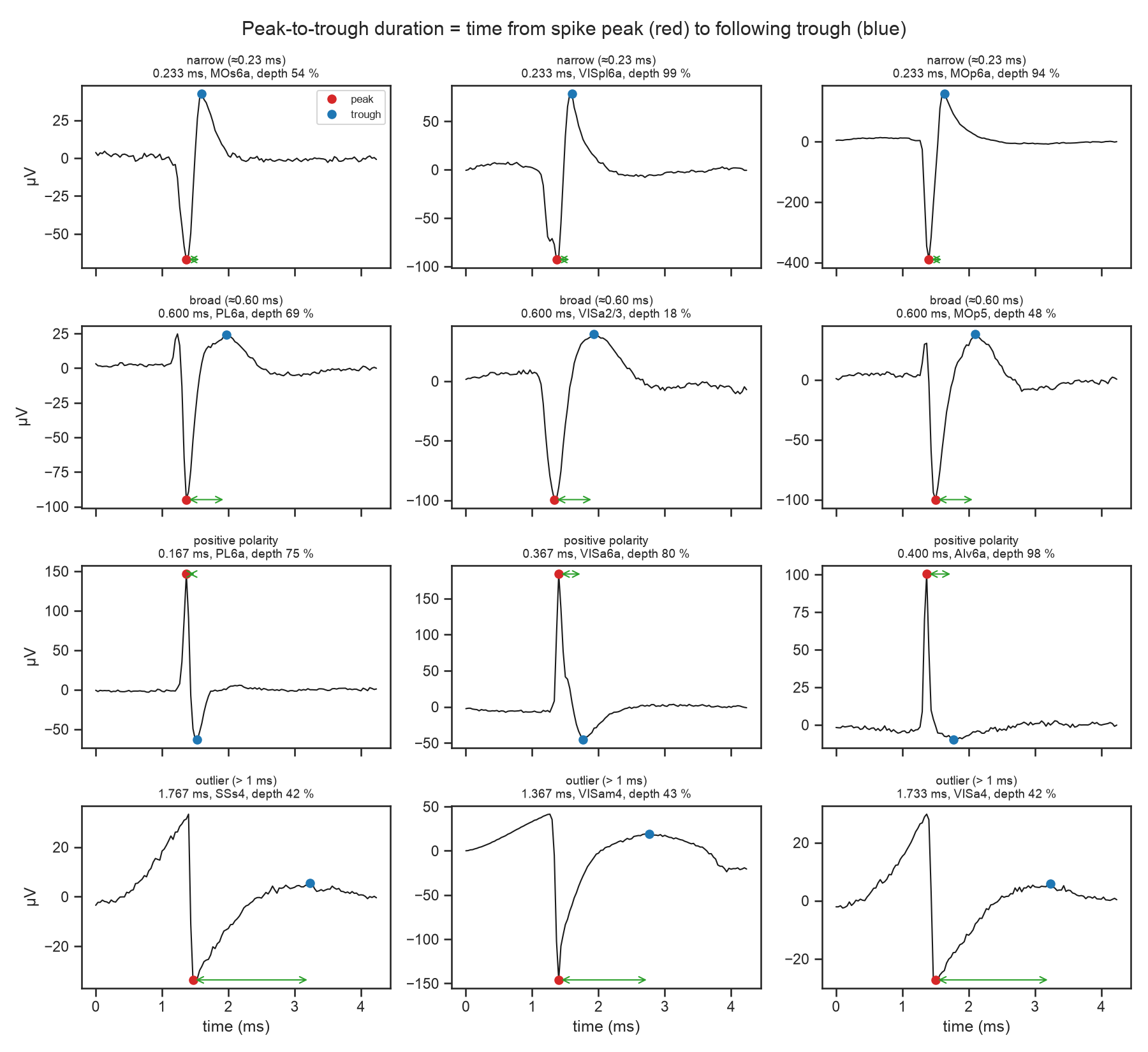
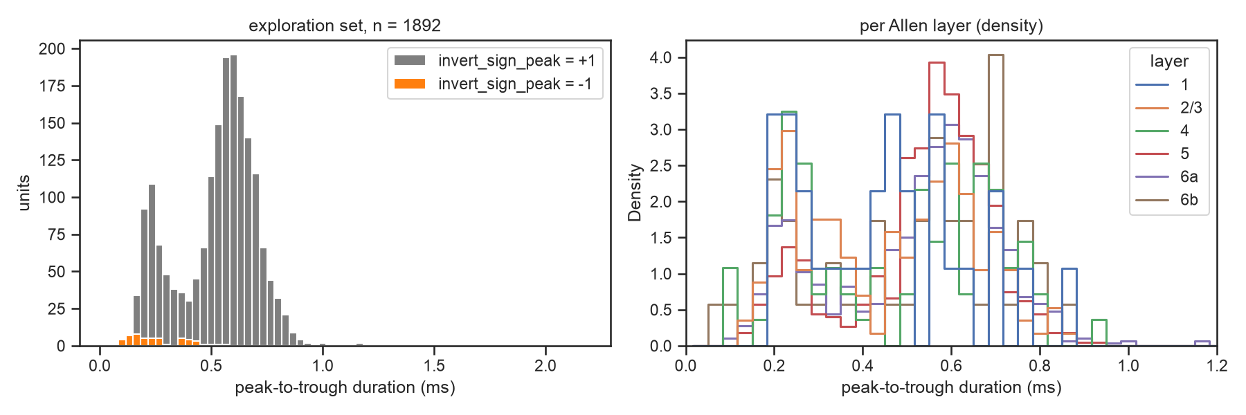
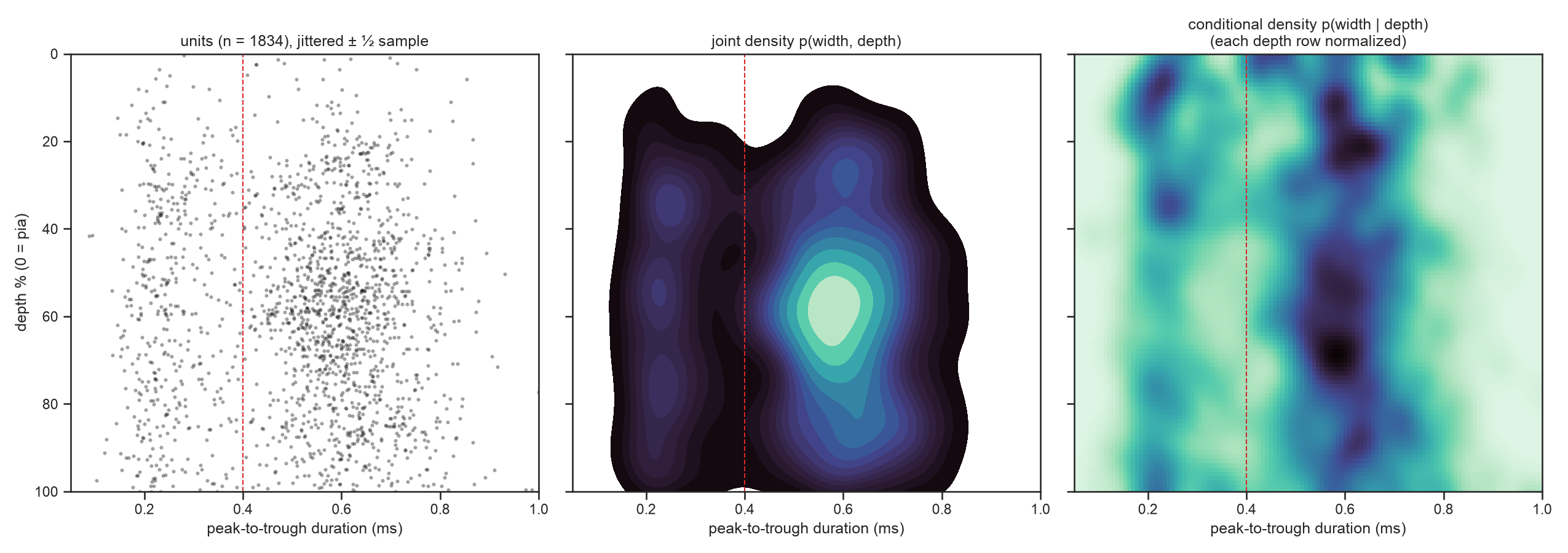
The width distribution is bimodal, with modes at ≈ 0.23 ms and ≈ 0.60 ms and a dip at ≈ 0.40 ms (Figure 2). Two waveform classes were excluded because the metric does not measure a somatic spike width for them:
- Positive-polarity units (2.7 %). For these the metric spans a positive peak and a negative trough, a likely axonal shape. They pile up below 0.3 ms and would inflate the narrow class.
- Units wider than 1 ms (0.3 %). Here the “trough” is a slow late hump (Figure 1, bottom row).
3.3 Cortical depth
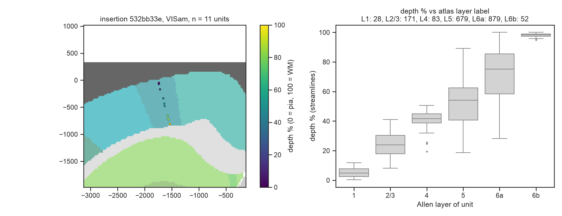
Cortical depth is the normalized position along the cortical streamline through each unit’s CCF coordinate (0 % = pia, 100 % = white matter), computed with iblatlas.streamlines.utils.xyz_to_depth. Depth increases monotonically with the Allen layer label of each unit (Figure 3). The layer 5 and 6a depth ranges overlap widely, consistent with localization error (~50–100 µm against ~1 mm of cortex) and with differences in layer thickness between areas.
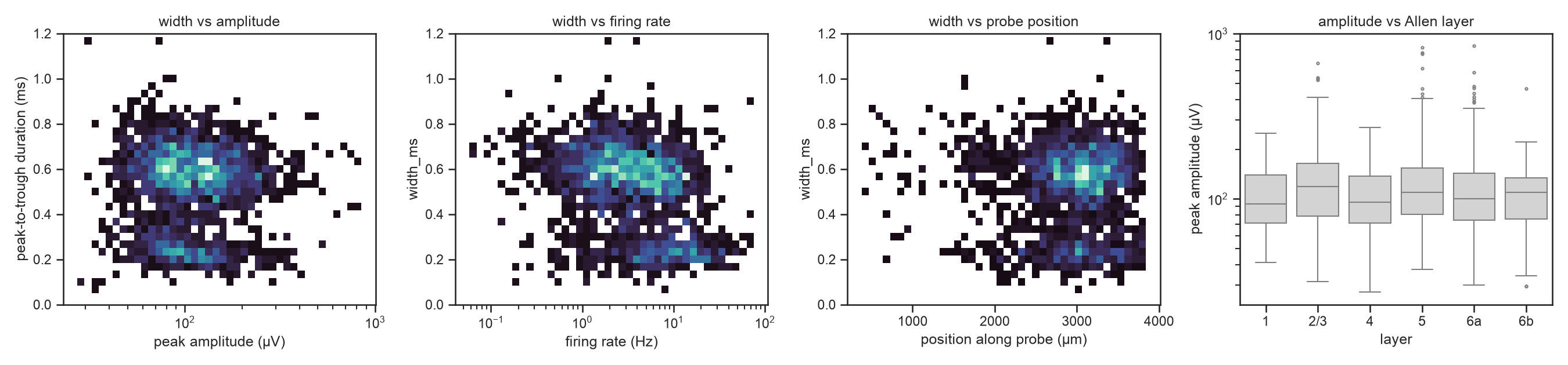
Width is not explained by recording geometry: it is nearly independent of spike amplitude (Spearman ρ = −0.04), and amplitude does not vary with layer (Figure 4). Narrow units fire faster (ρ = −0.31 between width and firing rate), as expected for fast-spiking interneurons.
3.4 Exploratory result: a non-monotonic profile
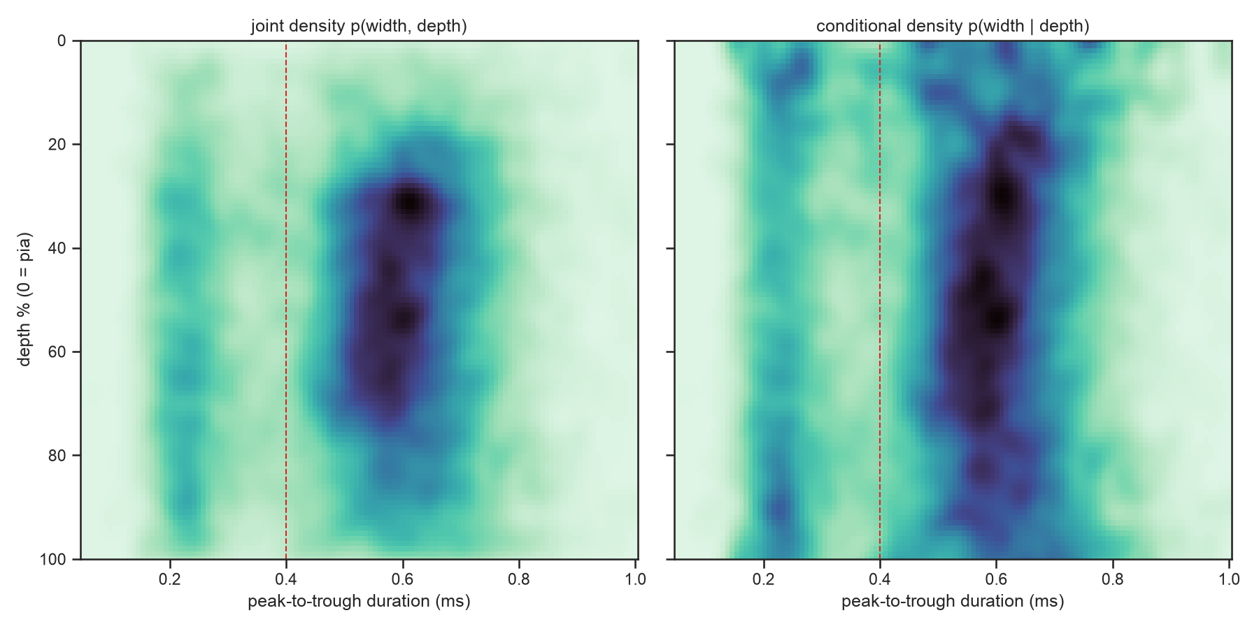
The joint distribution of width and depth (Figure 5) suggested that the narrow-unit fraction changes with depth without a monotonic trend. Per-mouse Spearman correlations between width and depth were centred on zero for every readout (median ρ between −0.02 and 0.03; Wilcoxon p > 0.5).
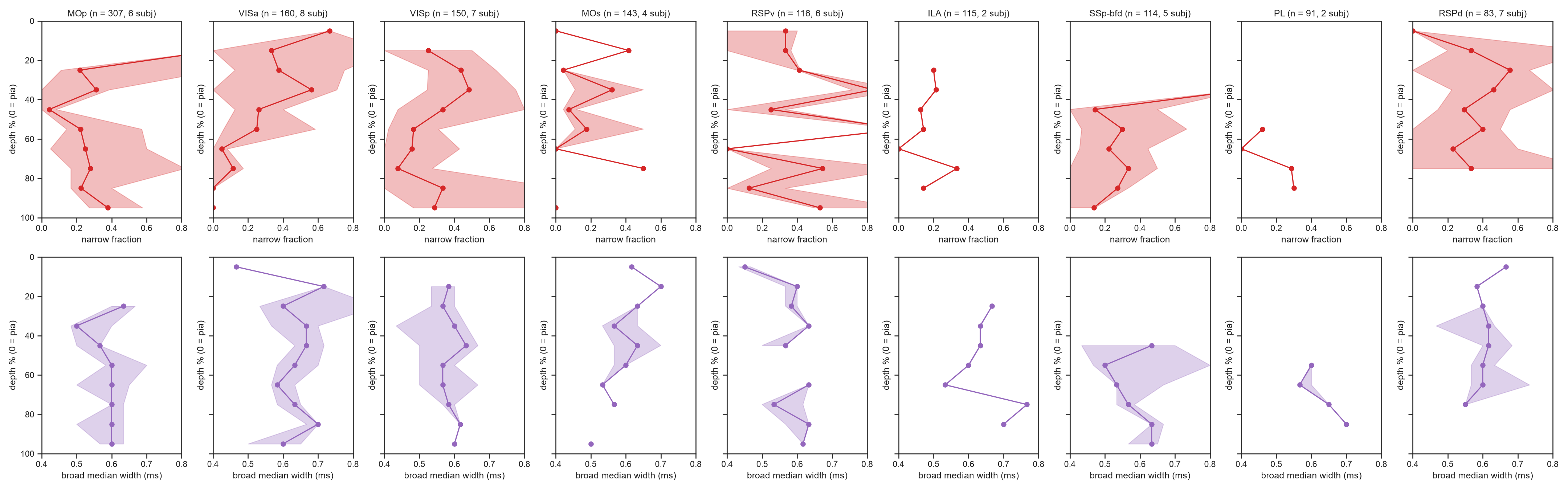
Depth profiles (Figure 6) showed a high narrow fraction superficially, a minimum at 40–70 % depth and a partial rebound deeper. Narrow/broad thresholds of 0.35, 0.40 and 0.45 ms gave parallel profiles, so 0.40 ms (the histogram dip) was retained. The median broad-unit width is coarse because of the 33 µs quantization, so the mean was used for confirmation. Per-region profiles (Figure 7) were too sparse to interpret with 2–8 mice per region.
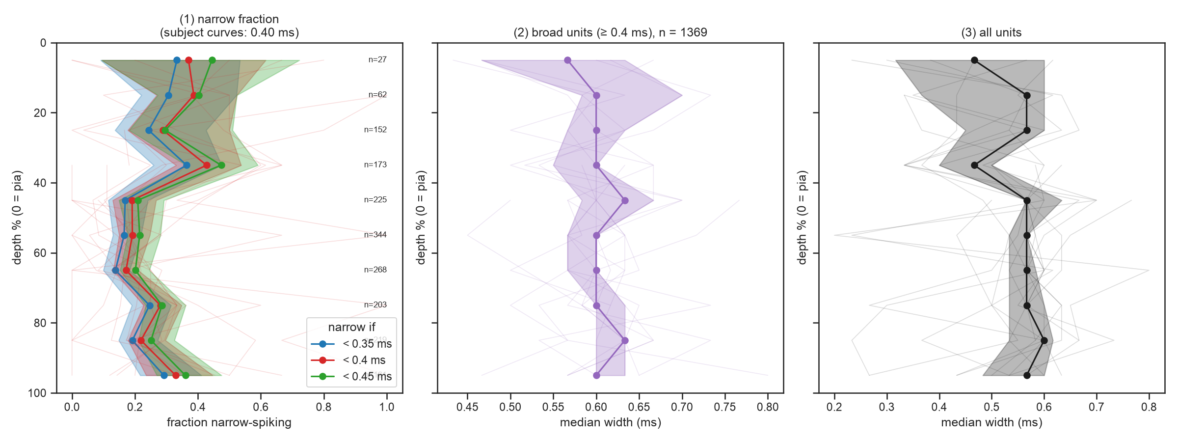
On the exploration set, band-based tests were strongly significant: within-insertion permutation χ² = 49.8, p = 2·10⁻⁴; superficial > mid in 10 of 11 mice, p = 0.003; broad width across bands p = 0.002.
3.5 Revised question
Among good isocortex units with somatic-like waveforms, does the fraction of narrow-spiking units (< 0.40 ms), and the width of broad-spiking units, differ between superficial (0–40 %), mid (40–70 %) and deep (70–100 %) cortical depth, within insertions?
4 Locked analysis plan
The following plan was locked before any analysis of the confirmation set. Exclusions, the 0.40 ms threshold and the band boundaries were all fixed.
| Test | Hypothesis | Null | |
|---|---|---|---|
| B (primary) | χ² of the 3 bands × narrow/broad table | narrow fraction differs across bands | depth bands permuted among units of the same insertion (10,000 permutations) |
| A (directional) | one-sided Wilcoxon signed-rank over mice with ≥ 5 units in both bands | narrow fraction superficial > mid | median per-mouse difference = 0 |
| C (secondary) | one-way F of broad-unit width across bands | broad width differs across bands | within-insertion permutation as in B |
Holm correction across the three tests, α = 0.05. Permuting within insertions keeps each insertion’s region, probe placement and narrow/broad mix, so only the depth arrangement within a probe is tested. Depth profiles, 2D KDE and per-region profiles were declared descriptive.
5 Results of confirmatory analysis
After exclusions, the confirmation set contained 10,754 units from 281 insertions and 93 mice.
| Depth band | Units | Narrow fraction | Mean broad width (ms) |
|---|---|---|---|
| superficial (0–40 %) | 3,424 | 0.213 | 0.622 |
| mid (40–70 %) | 4,383 | 0.184 | 0.603 |
| deep (70–100 %) | 2,947 | 0.250 | 0.616 |
- B (primary) is confirmed: the narrow fraction depends on depth within insertions (χ² = 46.2, Holm p = 3·10⁻⁴).
- C is confirmed: broad-unit width depends on depth (F = 30.8, Holm p = 3·10⁻⁴).
- A is not confirmed: the superficial-minus-mid difference was positive in 34 of 55 mice, but small (median 0.022; one-sided p = 0.08).
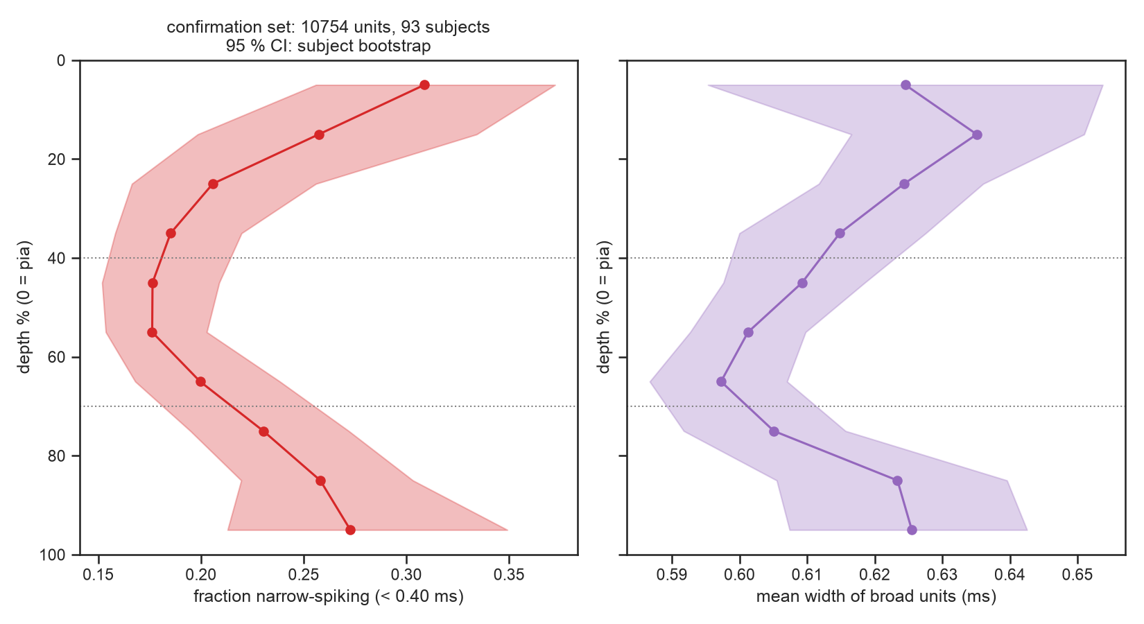
Both profiles are U-shaped, with a minimum at mid-depth (Figure 8). The narrow fraction falls from ≈ 0.31 just below the pia to ≈ 0.18 at 40–60 % depth, then rises to ≈ 0.27 near the white matter. Broad-unit width follows the same shape, from 0.635 ms to 0.597 ms and back to 0.625 ms: a difference of about one sample.
The 2D KDE (Figure 9) shows the narrow mode at ≈ 0.22 ms spread over all depths. The broad mode concentrates between 25 % and 75 % depth, and its conditional density is narrowest and shifted to shorter widths at mid-depth.
Test A failed for two reasons. First, the exploration set overestimated the superficial narrow fraction (0.37 against 0.21). Second, the locked 0–40 % band mixes the high 0–20 % range with the already-low 20–40 % range (Figure 8).
6 Post-hoc analyses
These analyses are descriptive and were not part of the locked plan.
Per region. The mid-depth dip in narrow fraction is visible in MOs, MOp, VISa, VISp and SSp-bfd. Several frontal and medial regions (ORBvl, ORBm, ACAd, PL) are flatter or noisy (Figure 10).

Per Allen layer. Narrow fraction by layer label: L1 0.32 (184 units), L2/3 0.27 (1,113), L4 0.26 (592), L5 0.17 (5,056), L6a 0.24 (3,561), L6b 0.25 (248).
7 Discussion
Main finding. Spike width varies with cortical depth, but not monotonically. Mid-depth units, mostly in layer 5, include the smallest fraction of narrow-spiking units and the narrowest broad-spiking units. Units near the pia or the white matter include more narrow units and slightly broader broad units. This is why per-mouse linear or rank correlations are null while band-based tests are significant. The effects are modest: Cramér’s V = 0.07 for the narrow fraction, and η² = 0.007 (≈ 30 µs) for broad-unit width.
Relation to prior knowledge. The scarcity of narrow units at mid-depth does not simply reflect interneuron density. Parvalbumin interneurons are abundant in layers 4–5 of many areas (Kim et al. 2017; Tremblay et al. 2016). A likely contributor is detection bias: large layer 5 pyramidal neurons produce large extracellular fields and are over-represented among sorted units, which lowers the narrow fraction there. The narrow excess just below the pia is consistent with layer 1 containing only interneurons. The rebound near the white matter may include axonal spikes or narrow-spiking deep pyramidal cells (Vigneswaran et al. 2011; Jia et al. 2019). These explanations were not tested here.
Caveats.
- Peak-to-trough duration is a proxy for cell type, not a label.
- CCF localization error is substantial relative to cortical thickness, and blurs the profile, especially at the edges.
- Sampling is dominated by layers 5–6 (≈ 80 % of units).
- The exclusion of positive-polarity units and units wider than 1 ms is a modelling choice.
- The within-insertion permutation treats units of one insertion as exchangeable. Oversplit clusters could make it anti-conservative; the subject-level test A guards against this but did not reach significance.
- Band boundaries were chosen on the exploration set and turned out to be poorly placed for the directional contrast.
Lessons for future analyses.
- A 24-mouse exploration set gave inflated effect sizes: Cramér’s V 0.17 against 0.07; rank-biserial 0.94 against 0.22. Directional contrasts locked on band boundaries chosen from noisy exploratory profiles are fragile. An omnibus test (B) was the robust choice.
- Shape-free tests are needed for non-monotonic profiles; correlation-based tests would have missed this effect.
- Stored waveform features need polarity and outlier checks before use.
8 Statistical information
Permutation p-values are bounded below by 1/(N + 1) ≈ 10⁻⁴. Holm correction was applied across the three confirmatory tests.
| Test | Figure | Comparison | Set | Statistic | df | n | p (Holm) | Effect size |
|---|---|---|---|---|---|---|---|---|
| B: χ² with within-insertion permutation null (10,000 permutations) | Figure 8 | narrow/broad × 3 depth bands | confirmation | χ² = 46.2 | 2 | 10,754 units, 281 insertions | 3·10⁻⁴ | Cramér’s V = 0.066 |
| A: Wilcoxon signed-rank, one-sided | Figure 8 | narrow fraction superficial > mid, per mouse | confirmation | W = 602 | – | 55 mice | 0.080 | rank-biserial r = 0.22; median diff = 0.022 |
| C: one-way F with within-insertion permutation null (10,000 permutations) | Figure 8 | broad-unit width across 3 depth bands | confirmation | F = 30.8 | (2, 8476) | 8,479 broad units | 3·10⁻⁴ | η² = 0.0072 |
| B (exploratory) | Figure 6 | as B | exploration | χ² = 49.8 | 2 | 1,834 units | 2·10⁻⁴ (unadjusted) | Cramér’s V = 0.165 |
| A (exploratory, two-sided) | Figure 6 | as A | exploration | W = 2 | – | 11 mice | 0.003 (unadjusted) | rank-biserial r = 0.94 |
| C (exploratory) | Figure 6 | as C | exploration | F = 9.48 | (2, 1366) | 1,369 broad units | 0.002 (unadjusted) | η² = 0.014 |
| Spearman per mouse + Wilcoxon (exploratory) | Figure 6 | width or narrow indicator vs depth | exploration | median ρ −0.02 to 0.03 | – | 16 mice | > 0.5 (unadjusted) | – |